Hourly electricity demand forecast and battery peak-shaving schedule
We forecast hourly electricity demand (MW) for each of 5 balancing authorities 7 days (168 hours) ahead from a public dataset. In testing on past data, the selected method (the AI forecasting model) was off by 5.7% of actual volume on average, 21% less error than repeating the same hour the day before. The grid operators' own day-ahead forecast did better, with 3% error.
Read this first
- The costs and limits in the plan (series, power mw, energy mwh, round trip efficiency, capacity price, off peak price, peak price, peak hours, timezone, degradation cost) are example values chosen to show the method. With your business, we use your numbers.
The request
"Forecast our hourly electricity demand for the next 7 days and show how you compare to our current day-ahead forecast."
The forecast
We expect electricity demand (MW) to average 85,040 over the next 168 hours for PJM, the largest series, peaking at about 93,910 on Fri, Oct 2, 12 AM.
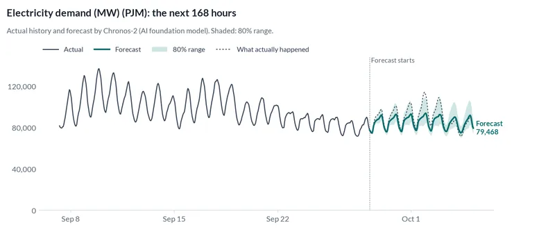
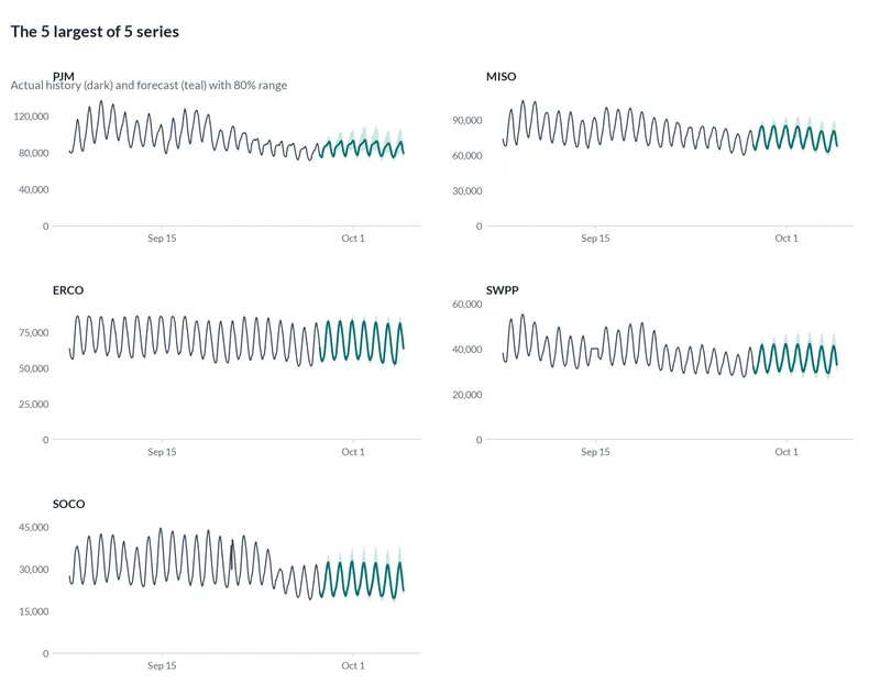
How accurate was it?
We hid the most recent stretch of history, forecast it using only what came before, and compared with what really happened. We did that 5 times, each time 7 days (168 hours) ahead, for every method below. The typical error is the share of actual volume the forecast missed by, added up across all 5 balancing authorities.
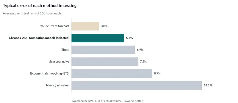
The selected method, an AI forecasting model that was not trained on this data, was off by 5.7% on average, against 7.2% for simply repeating the same hour the day before.
| Method | Kind | Typical error | Actual inside 80% range |
|---|---|---|---|
| AI forecasting model Selected | AI | 5.7% | 73% |
| Theta method | Classic | 6.9% | 100% |
| Repeat last season | Simple rule | 7.2% | 86% |
| Exponential smoothing | Classic | 8.7% | 69% |
| Repeat the last value | Simple rule | 14.1% | 92% |
| Current forecast | Current forecast | 3% | n/a |
The existing forecast was more accurate
The grid operators' own day-ahead forecast had 3% typical error, against 5.7% for ours. It is issued about a day ahead, while our test forecasts look up to 7 days ahead, so the comparison favors it.
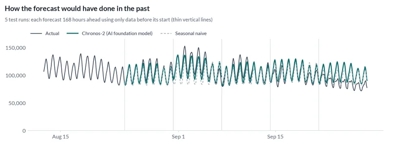
Reality check on data no model saw
Before running anything, we set aside the final 839 hours of the data (from 2026-09-28). Nothing in the testing above or the method choice could see them. Here is how every method did on that stretch.
The selected method was the most accurate here too, with 7% error.
| Method | Typical error |
|---|---|
| AI forecasting model Selected | 7% |
| Theta method | 9% |
| Repeat last season | 9.9% |
| Exponential smoothing | 10.6% |
| Repeat the last value | 13.2% |
The plan
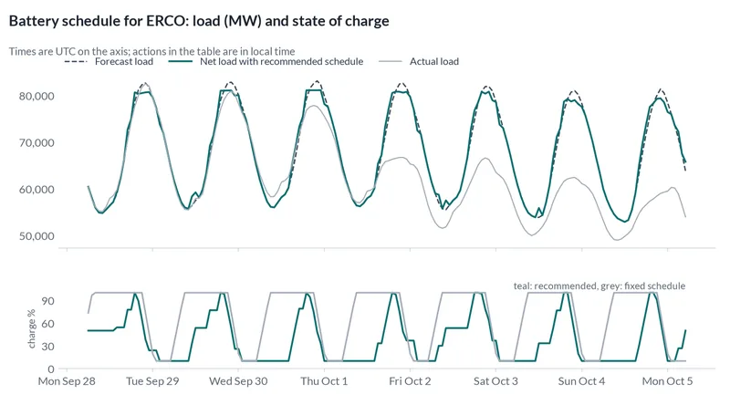
Recommended: charge in low-load, low-price hours and discharge into the forecast peaks. Expected peak 81,562 MW instead of 83,562 MW without the battery. Expected value this week $7.14M, against $4.12M for a fixed daily schedule (charge 01:00 to 05:00, discharge 17:00 to 21:00).
Why this schedule: the highest hour of the week sets the capacity cost ($2,000 per MW), so the battery is saved for the hours the forecast says will be the peak, and charged when load and prices are low. A fixed daily schedule discharges every evening whether or not that is where the peak falls.
Expected outcome: peak cut by 2,000 MW (fixed schedule: 360 MW); savings versus no battery $7.14M.
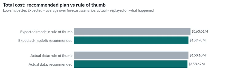
Reality check: this plan was made as of Sep 28, 2026 without seeing later data. Replayed on what actually happened, it cost $158.67M against $160.10M for the rule of thumb: a measured saving of $1.43M (29%).
Plan against the rule of thumb
The rule of thumb here is a fixed daily schedule (charge 01:00 to 05:00, discharge 17:00 to 21:00). We compare both ways: the expected cost over many possible futures from the forecast, and a replay of both plans on what actually happened.
| Comparison | Difference | Percent |
|---|---|---|
| Expected, over forecast scenarios | $3.02M | 73.4% |
| Replayed on what actually happened | $1.43M | 29.2% |
For a battery, percentages are relative to the value the rule of thumb creates, not to the total energy bill.
| Input | Value | Where it came from |
|---|---|---|
| Series | ERCO (name) | Example value |
| Power mw | 2,000 (MW) | Example value |
| Energy mwh | 8,000 (MWh) | Example value |
| Round trip efficiency | 0.87 (fraction) | Example value |
| Capacity price | 2,000 ($/MW) | Example value |
| Off peak price | 35 ($/MWh) | Example value |
| Peak price | 120 ($/MWh) | Example value |
| Peak hours | 16, 17, 18, 19, 20, 21 (local hours) | Example value |
| Timezone | America/Chicago (name) | Example value |
| Degradation cost | 10 ($/MWh) | Example value |
What the engine noticed in the data
- Forecast made as of Sep 28, 2026: 11,391 later rows were hidden from the models and used afterwards to check the forecast.
- 47,837 rows had no value for electricity demand (MW); treated as missing.
- Removed 111 rows with negative electricity demand (MW) (they look like errors).
Technical details
- Data
- U.S. EIA-930 Hourly Electric Grid Monitor - Balance files, United States. 5 balancing authorities, hourly, from 2026-05-31 to 2026-09-28.
- How we prepared the data
- Two 2026 half-year files (Jan to early Oct 2026). Keeps the 5 balancing authorities with the highest demand and the most recent 120 days (2,880 hours) of history. Uses UTC timestamps to avoid daylight-saving gaps and doubled hours. The authorities' own day-ahead forecast ('Demand Forecast (MW)') is scored as 'your current forecast'. Note that it is issued about a day ahead, while our test forecasts look up to 7 days ahead, so the comparison favors the day-ahead forecast. The last 7 days (Sep 28 to Oct 5, 2026, UTC) are hidden with as_of and used as the reality check. The battery example uses ERCO (Texas) only; timestamps are hour-ending UTC and are converted to Central time for the peak window. The battery size, prices and schedule rule are example values, not ERCOT tariffs.
- Testing
- 5 rolling tests, each 7 days (168 hours) ahead. Selection metric: WAPE (weighted absolute percentage error, the "typical error" above). Also reported: MASE 1.28 for the selected method.
- Methods
- Chronos-2 (AI foundation model), Theta, Seasonal naive, Exponential smoothing (ETS), Naive (last value), Your current forecast.
- Plan
- One-week battery schedule for peak shaving in ERCOT. Optimization status: ok, solver: optimal.
- Reproduce
- The case folder, spec and outputs are in the 4castPlannr repository under
cases/eia-930-hourly-demand/.
Data source and license
Source: U.S. Energy Information Administration, Form EIA-930 Hourly Electric Grid Monitor (accessed Oct 2026).
License: Public domain (U.S. Government work). Source: original data. The forecasts and charts on this page are derived from that data and carry the same attribution.
Have a decision like this?
This case is an example of energy and batteries for sites with batteries or demand charges. Send us your own export and question, and we will run the same tests on your data.